Load Data

import folium
import matplotlib.pyplot as plt
import pandas as pd
import plotly.express as px
import seaborn as sns

Load Data

data = pd.read_csv(
    "../data/tree_data/2015-street-tree-census-tree-data.csv",
    parse_dates=["created_at"],
    index_col="tree_id",
)

data.head()

	Unnamed: 0	block_id	created_at	tree_dbh	stump_diam	curb_loc	status	health	spc_latin	spc_common	...	boro_ct	state	latitude	longitude	x_sp	y_sp	council district	census tract	bin	bbl
tree_id
221864	19575	107688	2015-09-13	11	0	OnCurb	Alive	Poor	Pyrus calleryana	Callery pear	...	1013600	New York	40.773402	-73.947079	9.989077e+05	221052.5156	5.0	136.0	1051194.0	1.015800e+09
328163	172248	213992	2015-10-14	9	0	OnCurb	Alive	Good	Quercus bicolor	swamp white oak	...	3072600	New York	40.631616	-73.933963	1.002579e+06	169398.2032	45.0	726.0	3214207.0	3.077480e+09
690511	483212	214423	2016-08-31	25	0	OnCurb	Alive	Good	Platanus x acerifolia	London planetree	...	3095600	New York	40.635410	-73.909161	1.009462e+06	170786.3448	46.0	956.0	3225006.0	3.080200e+09
290017	103200	349008	2015-10-06	7	0	OnCurb	Alive	Good	Quercus palustris	pin oak	...	4071303	New York	40.728232	-73.849770	1.025888e+06	204626.9553	29.0	71303.0	4051256.0	4.021340e+09
40867	557989	108216	2015-06-29	10	0	OnCurb	Alive	Good	Styphnolobium japonicum	Sophora	...	1016001	New York	40.785596	-73.953476	9.971335e+05	225494.2784	4.0	16001.0	1047404.0	1.015060e+09

5 rows × 45 columns

Data info

data.info()

<class 'pandas.core.frame.DataFrame'>
Index: 10000 entries, 221864 to 612369
Data columns (total 45 columns):
 #   Column            Non-Null Count  Dtype         
---  ------            --------------  -----         
 0   Unnamed: 0        10000 non-null  int64         
 1   block_id          10000 non-null  int64         
 2   created_at        10000 non-null  datetime64[ns]
 3   tree_dbh          10000 non-null  int64         
 4   stump_diam        10000 non-null  int64         
 5   curb_loc          10000 non-null  object        
 6   status            10000 non-null  object        
 7   health            9545 non-null   object        
 8   spc_latin         9545 non-null   object        
 9   spc_common        9545 non-null   object        
 10  steward           2474 non-null   object        
 11  guards            1209 non-null   object        
 12  sidewalk          9545 non-null   object        
 13  user_type         10000 non-null  object        
 14  problems          3305 non-null   object        
 15  root_stone        10000 non-null  object        
 16  root_grate        10000 non-null  object        
 17  root_other        10000 non-null  object        
 18  trunk_wire        10000 non-null  object        
 19  trnk_light        10000 non-null  object        
 20  trnk_other        10000 non-null  object        
 21  brch_light        10000 non-null  object        
 22  brch_shoe         10000 non-null  object        
 23  brch_other        10000 non-null  object        
 24  address           10000 non-null  object        
 25  postcode          10000 non-null  int64         
 26  zip_city          10000 non-null  object        
 27  community board   10000 non-null  int64         
 28  borocode          10000 non-null  int64         
 29  borough           10000 non-null  object        
 30  cncldist          10000 non-null  int64         
 31  st_assem          10000 non-null  int64         
 32  st_senate         10000 non-null  int64         
 33  nta               10000 non-null  object        
 34  nta_name          10000 non-null  object        
 35  boro_ct           10000 non-null  int64         
 36  state             10000 non-null  object        
 37  latitude          10000 non-null  float64       
 38  longitude         10000 non-null  float64       
 39  x_sp              10000 non-null  float64       
 40  y_sp              10000 non-null  float64       
 41  council district  9902 non-null   float64       
 42  census tract      9902 non-null   float64       
 43  bin               9871 non-null   float64       
 44  bbl               9871 non-null   float64       
dtypes: datetime64[ns](1), float64(8), int64(11), object(25)
memory usage: 3.5+ MB

Missing values pie chart

missing_values_df = pd.DataFrame(data.isnull().mean() * 100, columns=["percantage"])
missing_values_df = missing_values_df[missing_values_df["percantage"] > 0]
missing_values_df

	percantage
health	4.55
spc_latin	4.55
spc_common	4.55
steward	75.26
guards	87.91
sidewalk	4.55
problems	66.95
council district	0.98
census tract	0.98
bin	1.29
bbl	1.29

fig = px.pie(missing_values_df, values="percantage", names=missing_values_df.index)
fig.update_layout(title="Процент пропущенных значений в данных", title_x=0.5)
fig.show()

features pairplot

data.head()

	Unnamed: 0	block_id	created_at	tree_dbh	stump_diam	curb_loc	status	health	spc_latin	spc_common	...	boro_ct	state	latitude	longitude	x_sp	y_sp	council district	census tract	bin	bbl
tree_id
221864	19575	107688	2015-09-13	11	0	OnCurb	Alive	Poor	Pyrus calleryana	Callery pear	...	1013600	New York	40.773402	-73.947079	9.989077e+05	221052.5156	5.0	136.0	1051194.0	1.015800e+09
328163	172248	213992	2015-10-14	9	0	OnCurb	Alive	Good	Quercus bicolor	swamp white oak	...	3072600	New York	40.631616	-73.933963	1.002579e+06	169398.2032	45.0	726.0	3214207.0	3.077480e+09
690511	483212	214423	2016-08-31	25	0	OnCurb	Alive	Good	Platanus x acerifolia	London planetree	...	3095600	New York	40.635410	-73.909161	1.009462e+06	170786.3448	46.0	956.0	3225006.0	3.080200e+09
290017	103200	349008	2015-10-06	7	0	OnCurb	Alive	Good	Quercus palustris	pin oak	...	4071303	New York	40.728232	-73.849770	1.025888e+06	204626.9553	29.0	71303.0	4051256.0	4.021340e+09
40867	557989	108216	2015-06-29	10	0	OnCurb	Alive	Good	Styphnolobium japonicum	Sophora	...	1016001	New York	40.785596	-73.953476	9.971335e+05	225494.2784	4.0	16001.0	1047404.0	1.015060e+09

5 rows × 45 columns

data_sample = data.sample(n=50000, replace=True, random_state=42)

num_cols = data_sample.select_dtypes(exclude="object").columns.to_list()
num_cols

['Unnamed: 0',
 'block_id',
 'created_at',
 'tree_dbh',
 'stump_diam',
 'postcode',
 'community board',
 'borocode',
 'cncldist',
 'st_assem',
 'st_senate',
 'boro_ct',
 'latitude',
 'longitude',
 'x_sp',
 'y_sp',
 'council district',
 'census tract',
 'bin',
 'bbl']

data_sample = data_sample.drop_duplicates()

data_sample.duplicated().sum()

sns.pairplot(data_sample[num_cols])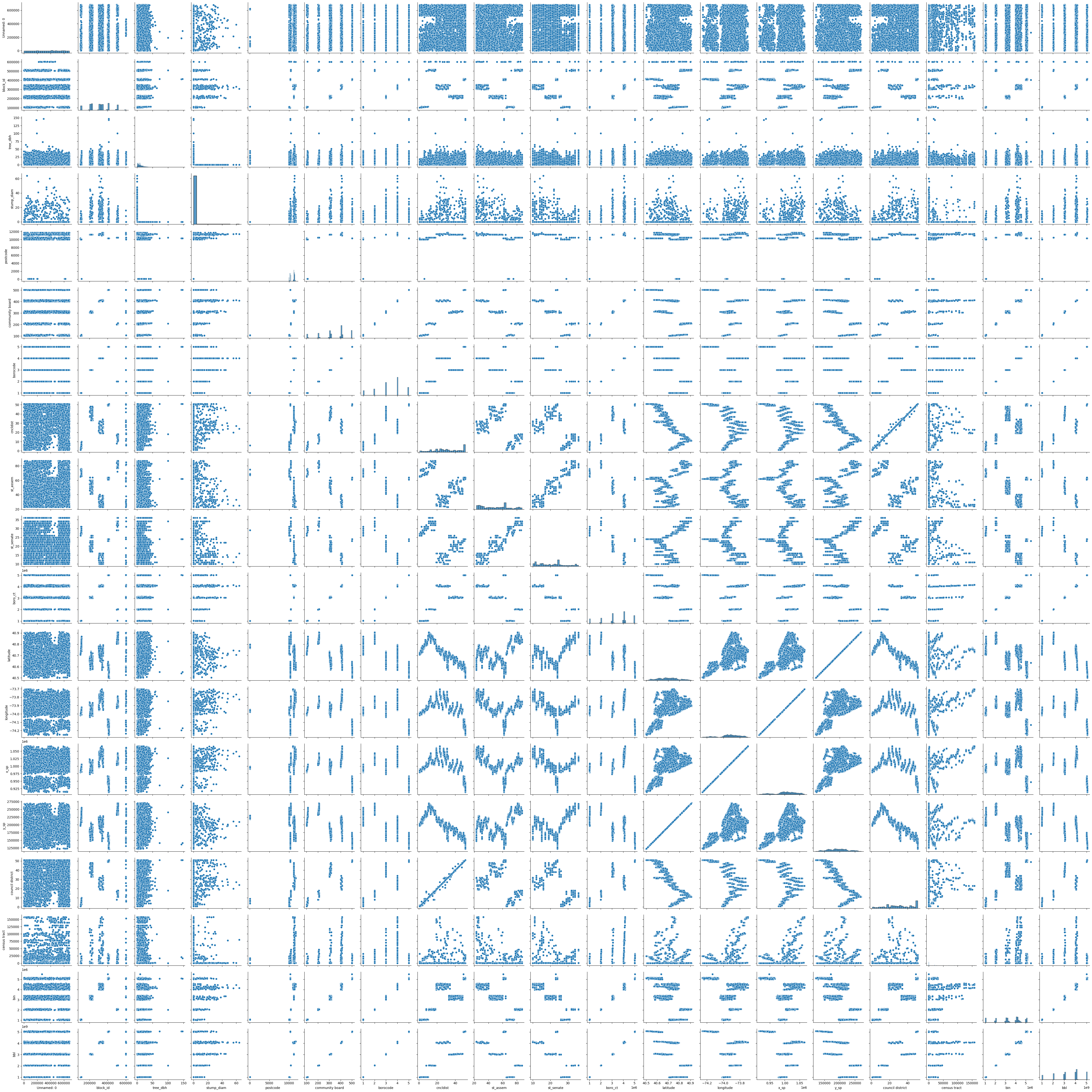

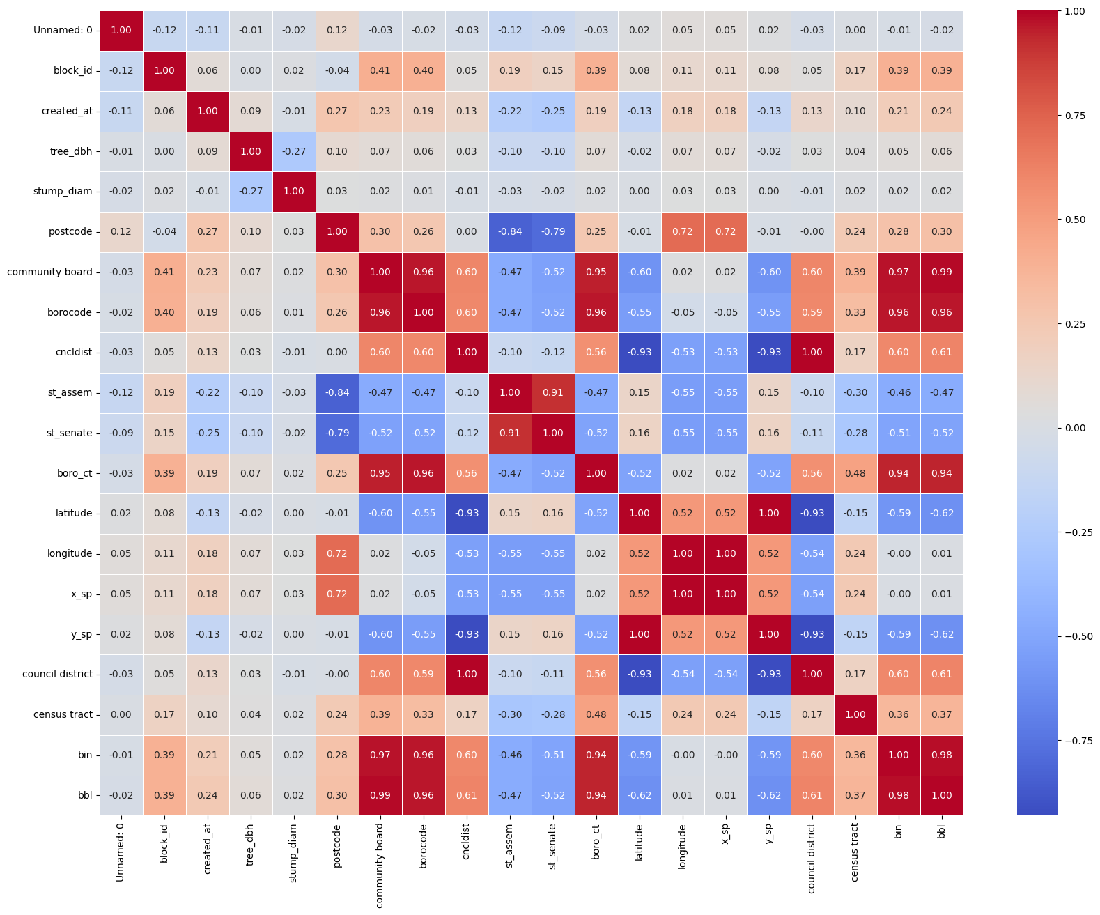
Correlation data

plt.figure(figsize=(20, 15))
sns.heatmap(
    data_sample[num_cols].corr(method="spearman"),
    annot=True,
    cmap="coolwarm",
    fmt=".2f",
    linewidths=0.5,
)

Tree mapping

# Make an empty map
m = folium.Map(location=[20, 0], tiles="OpenStreetMap", zoom_start=2)

import random

random_start = random.randint(0, 10000)
for i in range(0, 1000):
    folium.Marker(
        location=[data_sample.iloc[i]["latitude"], data_sample.iloc[i]["longitude"]],
        popup=data.iloc[i]["spc_latin"],
    ).add_to(m)

Make this Notebook Trusted to load map: File -> Trust Notebook